Conducting sensitivity analysis for survey weights
survey_weights.RmdIn the following vignette, we will walk through how to conduct a
sensitivity analysis for survey weights using
senseweight.
We will illustrate the analysis using a synthetically generated
dataset (available in data(poll.data)). The dataset is a
synthetic dataset comprising of 1000 individuals, where the outcome
variable Y indicates whether the individual supports a
policy position. When Y = 1, this implies that the
individual indicated support for a hypothetical candidate or policy
position, whereas 0 implies a lack of support. The dataset contains
common demographic covariates used in practice (age, education, gender,
race, party identification, and an indicator for whether an individual
is a born-again Christian).1
To load in the dataset:
data(poll.data)
poll.data |> head()
#>   Y age_buckets                educ gender  race         pid bornagain
#> 1 0      51to64             College    Men White Independent       Yes
#> 2 1      Over65           Post-grad  Women White    Democrat       Yes
#> 3 0      51to64 High School or Less    Men White Independent        No
#> 4 0      36to50 High School or Less    Men White  Republican        No
#> 5 1      51to64             College  Women White Independent       Yes
#> 6 0      Over65             College    Men White Independent        No
Setting up survey objects
The senseweight package builds on top of the
survey package to conduct sensitivity analysis. To start,
we will set up different survey objects for our analysis.
poll_srs <- svydesign(ids = ~ 1, data = poll.data)We have created a vector of population targets using a subset of the
2020 CES. It is in a locally stored vector pop_targets:2
print(pop_targets)
#>             (Intercept)       age_buckets36to50       age_buckets51to64
#>                   1.000                   0.212                   0.264
#>       age_bucketsOver65 educHigh School or Less           educPost-grad
#>                   0.236                   0.310                   0.114
#>        educSome college             genderWomen               raceBlack
#>                   0.360                   0.528                   0.114
#>            raceHispanic               raceOther               raceWhite
#>                   0.021                   0.034                   0.805
#>          pidIndependent                pidOther           pidRepublican
#>                   0.266                   0.075                   0.312
#>            bornagainYes
#>                   0.349
We will use raking as our weighting method of choice.
#Set up raking formula:
formula_rake <- ~ age_buckets + educ + gender + race + pid + bornagain

#PERFORM RAKING:
model_rake <- calibrate(
  design = poll_srs,
  formula = formula_rake,
  population = pop_targets,
  calfun = "raking",
  force = TRUE
)


rake_results <- svydesign( ~ 1, data = poll.data, weights = stats::weights(model_rake))
#Estimate from raking results:
weights = stats::weights(rake_results) * nrow(model_rake)

unweighted_estimate = svymean(~ Y, poll_srs, na.rm = TRUE)
weighted_estimate = svymean(~ Y, model_rake, na.rm = TRUE)
The unweighted survey estimate is 0.52.
print(unweighted_estimate)
#>   mean     SE
#> Y 0.52 0.0158
In contrast, the weighted survey estimate is 0.49.
print(weighted_estimate)
#>      mean     SE
#> Y 0.48981 0.0158
Summarizing sensitivity
With the survey objects, we can now generate our sensitivity
summaries. The senseweight package provides functions for
researchers to generate (1) robustness values; (2) benchmarking results;
and (3) bias contour plots. We walk through each of these below.
Robustness Value
The robustness value is a single numeric summary capturing how strong
a confounder has to be to change our research conclusion. The
summarize_sensitivity function will produce a table that
outputs the unweighted estimate, the weighted estimate, and the
robustness value corresponding to a threshold value
.
The threshold value corresponds to an estimate that would result in a
change in the substantive takeaway from a result. For example, in our
particular setting, we set the threshold value to be
,
which would imply that the proportion of individuals who support the
policy would change from a minority to a majority. The specification for
the threshold value is given by the b_star argument in the
summarize_sensitivity function.
summarize_sensitivity(estimand = 'Survey',
                      Y = poll.data$Y,
                      weights = weights,
                      svy_srs = unweighted_estimate,
                      svy_wt = weighted_estimate,
                      b_star = 0.5)
#>   Unweighted Unweighted_SE Estimate         SE   RV
#> 1       0.52    0.01580664 0.489811 0.01578579 0.02
We obtain a robustness value of 0.02. This implies that if the error from omitting a confounder is able to explain 2% of the variation in the oracle weights and 2% of the variation in the outcome, then this will be sufficient to push the survey estimate above the 50% threshold.
We can also choose to directly estimate the robustness value using
the robustness_value function:
robustness_value(estimate = 0.49,
                 b_star = 0.5,
                 sigma2 = var(poll.data$Y),
                 weights = weights)
#> [1] 0.0180977
Alternatively, researchers may be interested in setting to correspond to an estimate that is 2 standard deviations away from the original estimate. In this case, this would correspond to an estimate of approximately 0.52.
robustness_value(estimate = 0.49,
                 b_star = 0.52,
                 sigma2 = var(poll.data$Y),
                 weights = weights)
#> [1] 0.05331068
In this case, the the error from omitting a confounder would need to explain 5% of the variation in the oracle weights and 5% of the variation in the outcome to push the survey estimate above the 52% threshold.
Benchmarking
To help reason about the plausibility of potential confounders, we can also perform benchmarking. Benchmarking allows researchers to estimate the magnitude of sensitivity parameters that correspond to an omitted confounder that has equivalent confounding strength to an observed covariate.
To benchmark a single covariate, we can use the
benchmark_survey function:
benchmark_survey('educ',
                 formula = formula_rake,
                 weights = weights,
                 population_targets = pop_targets,
                 sample_svy = poll_srs,
                 Y = poll.data$Y)
#>   variable R2_benchmark rho_benchmark        bias
#> 1     educ    0.2237989    0.02030063 0.005968458
Alternatively, we can choose to benchmark all the covariates by
calling run_benchmarking. To specify that we are in a
survey setting, we set estimand = "Survey" in the
function:
covariates = c("age_buckets", "educ", "gender", "race",
               "educ", "pid", "bornagain")

benchmark_results = run_benchmarking(estimate = 0.49,
                 RV = 0.02,
                 formula = formula_rake,
                 weights = weights,
                 Y = poll.data$Y,
                 sample_svy = poll_srs,
                 population_targets = pop_targets,
                 estimand= "Survey")
print(benchmark_results)
#>      variable R2_benchmark rho_benchmark  bias     MRCS k_sigma_min k_rho_min
#> 1 age_buckets         0.39          0.04  0.02    31.46        0.05      3.93
#> 2        educ         0.22          0.02  0.01    82.10        0.09      6.97
#> 3      gender         0.07         -0.08 -0.01   -42.33        0.27     -1.88
#> 4        race         0.15          0.01  0.00   334.23        0.14     21.76
#> 5         pid         0.04          0.00  0.00 -1460.14        0.50    -46.86
#> 6   bornagain         0.04          0.05  0.01    93.05        0.47      3.09
The function will automatically return the benchmarking results, as well as a measure called the minimum relative confounding strength (MRCS), which calculates how much stronger (or weaker) an omitted confounder must be, relative to an observed covariate, in order to a be a killer confounder.
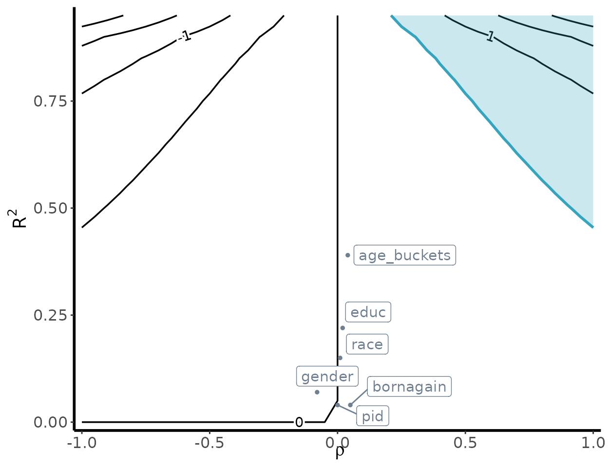
Bias contour plot
To visualize the sensitivity of our underlying estimates, we can
generate a bias contour plot using the following
contour_plot function:
contour_plot(varW = var(weights),
             sigma2 = var(poll.data$Y),
             killer_confounder = 0.5,
             df_benchmark = benchmark_results,
             shade = TRUE,
             label_size = 4)