Bias Contour Plots

Generates bias contour plots to aid with sensitivity analysis

Usage

contour_plot(
  varW,
  sigma2,
  killer_confounder,
  df_benchmark,
  benchmark = TRUE,
  shade = FALSE,
  shade_var = NULL,
  shade_fill = "#35a4bf",
  shade_alpha = 0.25,
  contour_width = 1,
  binwidth = NULL,
  label_size = 0.25,
  point_size = 1,
  nudge = 0.05,
  axis_text_size = 12,
  axis_title_size = 14,
  axis_line_width = 1,
  print = FALSE
)

Arguments

varW

Variance of the estimated weights

sigma2

Estimated variance of the outcome (i.e., stats::var(Y) for obervational setting; stats::var(tau) for generalization setting)#'

killer_confounder

Threshold for bias considered large enough to be a killer confounder. For example, if researchers are concerned about the bias large enough to reduce an estimated treatment effect to zero or change directional sign, set killer_confounder equal to the point estimate.

df_benchmark

Data frame containing formal benchmarking results. The data.frame must contain the columns variable (for the covariate name), R2_benchmark, and rho_benchmark.

benchmark

Flag for whether or not to display benchmarking results (benchmark = TRUE if we want to add benchmarking results to plot, benchamrk=FALSE otherwise). If set to TRUE, df_benchmark must contain valid benchmarking results.

shade

Flag for whether or not a specific benchmarking covariate (or set of benchmarked covariates) should be shaded a different color (shade = TRUE indicates that we want to highlight specific variables)

shade_var

If shade = TRUE, this contains either a vector containing the variables we want to highlight

shade_fill

Color to fill the highlighted variables. Default is set to "#35a4bf".

shade_alpha

Alpha value for the fill color. Default is set to 0.25.

contour_width

Width of the contour lines. Default is set to 1.

binwidth

If set to a numeric value, the function will generate a contour plot with the specified binwidth. Default is set to NULL.

label_size

Size of the labels. Default is set to 0.25.

point_size

Size of the points. Default is set to 1.

nudge

Nudge value for the labels. Default is set to 0.05.

axis_text_size

Size of the axis text. Default is set to 12.

axis_title_size

Size of the axis title. Default is set to 14.

axis_line_width

Width of the axis lines. Default is set to 1.

print

If set to TRUE, the function will return a list with two elements: plot which contains the generated bias contour plot, and data, which provides the data.frame for generating the contour plot. If set to FALSE, the function will simply generate the bias contour plot. Default is set to FALSE.

Value

A ggplot2 object, containing the bias contour plot

Examples

# For the external validity setting: 
data(jtpa_women)
site_name <- "NE"
df_site <- jtpa_women[which(jtpa_women$site == site_name), ]
df_else <- jtpa_women[which(jtpa_women$site != site_name), ]

# Estimate unweighted estimator:
model_dim <- estimatr::lm_robust(Y ~ T, data = df_site)
PATE <- coef(lm(Y ~ T, data = df_else))[2]
DiM <- coef(model_dim)[2]
# Generate weights using observed covariates:
df_all <- jtpa_women
df_all$S <- ifelse(jtpa_women$site == "NE", 1, 0)
model_ps <- WeightIt::weightit(
  (1 - S) ~ . - site - T - Y, 
  data = df_all, method = "ebal", estimand = "ATT"
)
weights <- model_ps$weights[df_all$S == 1]
# Estimate IPW model:
model_ipw <- estimatr::lm_robust(Y ~ T, data = df_site, weights = weights)
ipw <- coef(model_ipw)[2]
# Estimate bound for var(tau):
vartau <- var(df_site$Y[df_site$T == 1]) - var(df_site$Y[df_site$T == 0])
RV <- robustness_value(estimate = ipw, b_star = 0, sigma2 = vartau, weights = weights)

# Select weighting variables:
weighting_vars <- names(df_all)[which(!names(df_all) %in% c("site", "S", "Y", "T"))]

# Run benchmarking:
df_benchmark <- run_benchmarking(
  weighting_vars = weighting_vars,
  data = df_all[, -1],
  treatment = "T", outcome = "Y", selection = "S",
  estimate = ipw,
  RV = RV, sigma2 = vartau,
  estimand = "PATE"
)
# Generate bias contour plot:
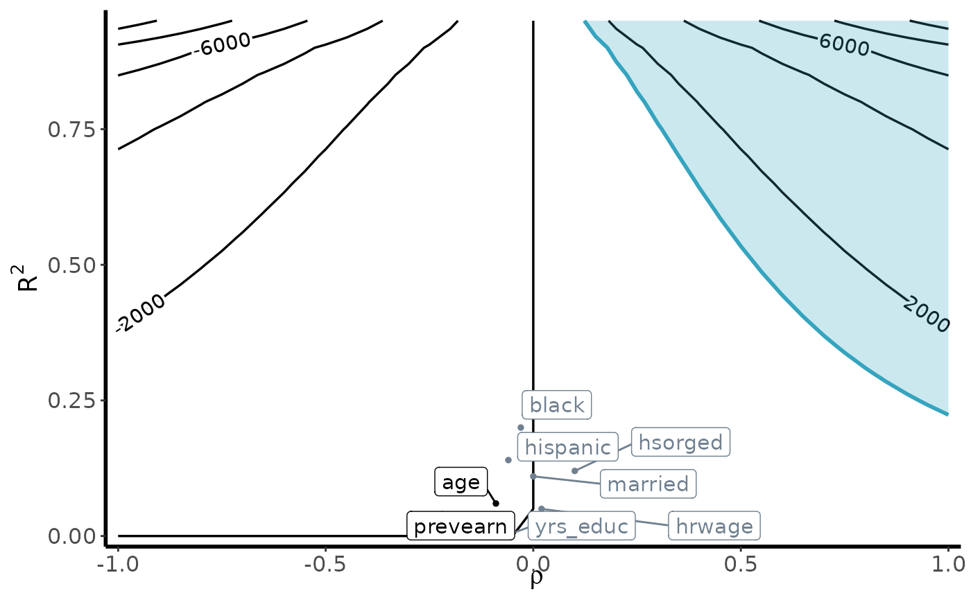
contour_plot(
var(weights), vartau, ipw, df_benchmark,
benchmark = TRUE, shade = TRUE,
shade_var = c("age", "prevearn"),
label_size = 4
)