Sensitivity analysis for external validity • senseweight

In the following vignette, we will walk through a basic example of how to conduct a sensitivity analysis for external validity using senseweight. We will use a subset of the JTPA data.

library(senseweight)
library(ggplot2)
# Load in JTPA data:
data(jtpa_women)

# Summarize sites
jtpa_women |>
  dplyr::group_by(site) |>
  dplyr::summarize(
    length(prevearn),
    dplyr::across(
      c(prevearn, age, married, hrwage, black, hispanic, hsorged, yrs_educ), 
      mean
    )
  )
#> # A tibble: 16 × 10
#>    site  `length(prevearn)` prevearn   age married hrwage   black hispanic
#>    <chr>              <int>    <dbl> <dbl>   <dbl>  <dbl>   <dbl>    <dbl>
#>  1 CC                   524    1855.  32.1  0.219    479. 0.101    0.693  
#>  2 CI                   190    2250.  33.5  0.253    458. 0.0684   0.0105 
#>  3 CV                   788    2192.  33.6  0.278    455. 0.173    0.00635
#>  4 HF                   234    1997.  31.6  0.184    455. 0.432    0.0342 
#>  5 IN                  1392    3172.  34.9  0.193    466. 0.243    0.0194 
#>  6 JC                    81    2564.  30.6  0.136    531. 0.642    0.247  
#>  7 JK                   353    1928.  30.0  0.113    453. 0.912    0      
#>  8 LC                   485    3039.  33.9  0.258    464. 0.0165   0.165  
#>  9 MD                   177    2915.  34.6  0.181    480. 0.367    0      
#> 10 MN                   179    2215.  37.6  0.352    454. 0.00559  0.0782 
#> 11 MT                    38    1680.  33.8  0.395    474. 0        0.0526 
#> 12 NE                   636    2161.  31.7  0.0975   477. 0.511    0.0377 
#> 13 OH                    74    2568.  34.6  0.324    486. 0.0135   0      
#> 14 OK                    87    2320.  37.3  0.126    586. 0.759    0.0805 
#> 15 PR                   463    1783.  32.8  0.0842   506. 0.268    0.378  
#> 16 SM                   401    2997.  32.2  0.284    429. 0.0200   0.00249
#> # ℹ 2 more variables: hsorged <dbl>, yrs_educ <dbl>

Assume researchers are interested in generalizing the results from the site of Omaha, Nebraska to the other 15 experimental sites:

site_name <- "NE"
df_site <- jtpa_women[which(jtpa_women$site == site_name), ]
df_else <- jtpa_women[which(jtpa_women$site != site_name), ]

# Estimate unweighted estimator:
model_dim <- estimatr::lm_robust(Y ~ T, data = df_site)
PATE <- coef(lm(Y ~ T, data = df_else))[2]
DiM <- coef(model_dim)[2]

# Generate weights using observed covariates:
df_all <- jtpa_women
df_all$S <- ifelse(jtpa_women$site == "NE", 1, 0)
model_ps <- WeightIt::weightit(
  (1 - S) ~ . - site - T - Y, 
  data = df_all, method = "ebal", estimand = "ATT"
)
weights <- model_ps$weights[df_all$S == 1]

# Estimate IPW model:
model_ipw <- estimatr::lm_robust(Y ~ T, data = df_site, weights = weights)
ipw <- coef(model_ipw)[2]

# Estimate bound for var(tau):
m <- sqrt(stats::var(df_site$Y[df_site$T == 1]) / stats::var(df_site$Y[df_site$T == 0]))
# Since m > 1:
vartau <- stats::var(df_site$Y[df_site$T == 1]) - stats::var(df_site$Y[df_site$T == 0])

Sensitivity Summary Measures

Robustness value

We can generate the sensitivity summary measures using the summarize_sensitivity function:

summarize_sensitivity(
  weights = weights, 
  Y = df_site$Y, 
  Z = df_site$T, 
  sigma2 = vartau, 
  estimand = "PATE"
)
#>   Unweighted Unweighted_SE Estimate     SE   RV sigma_tau_bound cor_w
#> Z    1107.35        982.65  1356.66 1417.3 0.36          2897.9  0.07

The summarize_sensitivity function defaults to evaluating the robustness value at q=1, indicating a robustness value, relative to a bias equal to the point estimate. Researchers can specify different values for q in the function. In the generalization setting, researchers can modify the sigma2 bound and posit their own values for a plausible bound (given substantive justification). With no specification, sigma2 will be automatically calculated to be bound by var(Y(1)) + var(Y(0)).

RV = robustness_value(estimate = ipw, b_star = 0, sigma2 = vartau, weights = weights)
print(RV)
#> [1] 0.4113622

Benchmarking

# Select weighting variables:
weighting_vars = names(df_all)[which(!names(df_all) %in% c("site", "S", "Y", "T"))]

# Run bechmarking:
df_benchmark <- run_benchmarking(
  weighting_vars = weighting_vars,
  data = df_all[, -1],
  treatment = "T", outcome = "Y", selection = "S",
  estimate = ipw,
  RV = RV, sigma2 = vartau,
  estimand = "PATE"
)


print(df_benchmark)
#>   variable R2_benchmark rho_benchmark    bias    MRCS k_sigma_min k_rho_min
#> 1 prevearn         0.04         -0.22 -115.00  -11.80        9.99     -2.92
#> 2      age         0.06         -0.09  -55.45  -24.47        6.91     -7.37
#> 3  married         0.11          0.00   -2.52 -539.33        3.82   -224.19
#> 4   hrwage         0.05          0.02   13.51  100.40        8.32     27.40
#> 5    black         0.20         -0.03  -33.11  -40.97        2.03    -24.72
#> 6 hispanic         0.14         -0.06  -62.63  -21.66        3.01    -10.30
#> 7  hsorged         0.12          0.10   95.06   14.27        3.51      6.22
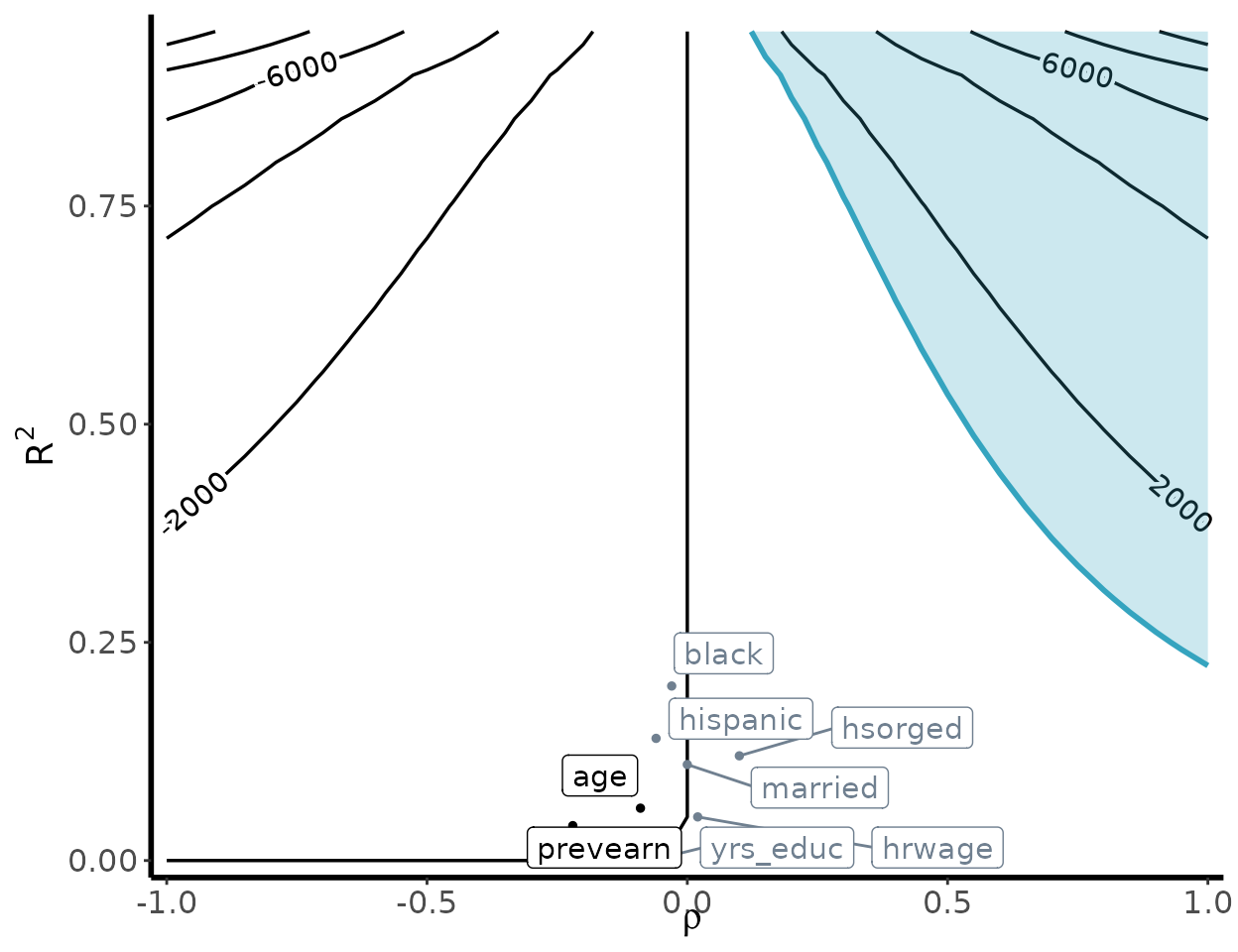
#> 8 yrs_educ         0.00         -0.07   -5.23 -259.49      408.90     -9.85

Bias Contour Plot

contour_plot(
  var(weights), vartau, ipw, df_benchmark,
  benchmark = TRUE, shade = TRUE,
  shade_var = c("age", "prevearn"),
  label_size = 4
)